IBEA
Indicator-based selection turns pairwise objective comparisons into fitness [1]. Here the additive epsilon indicator drives search; the indicator chosen for selection need not be the metric used to report final quality.
Goal: run the stable public API in VAMOS 1.4.0, interpret its returned population, and identify which settings control this mechanism.
Capability matrix · Exact configuration reference · Setup and recorded evidence
Run the example
Prerequisite: complete T01 and the coverage setup. The protocol uses ZDT1, 10 real variables, 2 objectives, population 40; 400 evaluations; NumPy; seed 42. Initial evaluations count towards the budget. Settings are illustrative, not tuned.
python ibea.py
python ibea.py --output ibea-local.svg
The second command reruns the same protocol and requires Matplotlib. Use a new filename.
Complete runnable script
"""Verified VAMOS 1.4.0 lesson: ibea. See coverage-setup for dependencies."""


def execute_example(problem, algorithm, config, budget, seed=42, engine="numpy"):
    import numpy as np

    from vamos import OptimizationResult, optimize

    result = optimize(problem, algorithm=algorithm, algorithm_config=config, max_evaluations=budget, seed=seed, engine=engine)
    G = result.data.get("G")
    if getattr(problem, "n_constraints", 0) and G is None:
        raise ValueError("Declared constraints are missing from the returned result.")
    feasible_rows = np.arange(len(result.F)) if G is None else np.flatnonzero(np.all(G <= 0, axis=1))
    if len(feasible_rows):
        feasible = OptimizationResult({"X": result.X[feasible_rows], "F": result.F[feasible_rows]})
        front, local = feasible.front(return_indices=True)
        front_rows = feasible_rows[local]
    else:
        front, front_rows = np.empty((0, problem.n_obj)), np.empty(0, dtype=int)
    print(f"Algorithm: {algorithm}; encoding: {problem.encoding}; backend: {engine}; seed: {seed}")
    print(f"Returned X: {result.X.shape}; F: {result.F.shape}; result mode: population")
    print(f"Feasible rows: {len(feasible_rows)}/{len(result.F)}; feasible non-dominated rows: {len(front)}")
    print(f"Evaluations: {result.data['evaluations']}")
    return {
        "problem": problem,
        "algorithm": algorithm,
        "config": config,
        "result": result,
        "feasible_rows": feasible_rows,
        "front": front,
        "front_rows": front_rows,
    }


def run_ibea(budget=400):
    from vamos.algorithms import IBEAConfig
    from vamos.problems import ZDT1

    problem = ZDT1(n_var=10)
    config = (
        IBEAConfig.builder()
        .pop_size(40)
        .crossover("sbx", prob=1.0, eta=20.0)
        .mutation("pm", prob=1.0 / problem.n_var, eta=20.0)
        .selection("tournament")
        .indicator("eps")
        .kappa(1.0)
        .result_mode("population")
        .build()
    )
    return execute_example(problem, "ibea", config, budget)


def plot_example(data, output):
    from pathlib import Path

    import matplotlib

    matplotlib.use("Agg")
    import matplotlib.pyplot as plt
    import numpy as np

    output = Path(output)
    if output.exists():
        raise FileExistsError(f"Choose a new figure filename: {output}")
    if output.suffix.lower() != ".svg":
        raise ValueError("Use an .svg output filename.")
    f = data["result"].F
    with plt.rc_context({"svg.hashsalt": "vamos-coverage", "svg.fonttype": "none"}):
        fig = plt.figure(figsize=(7, 4.5), layout="constrained")
        if f.shape[1] == 3:
            ax = fig.add_subplot(projection="3d")
            ax.scatter(*f.T, c="#007f7a", s=22)
            ax.set(xlabel="f1", ylabel="f2", zlabel="f3")
            ax.set_box_aspect((1, 1, 0.85), zoom=0.85)
        else:
            ax = fig.add_subplot()
            ax.scatter(*f.T, c="#b6bec8", s=25, label="Returned population")
            if len(data["front"]):
                ax.scatter(*data["front"].T, c="#007f7a", s=30, label="Feasible non-dominated rows")
            labels = {
                "WeldedBeamDesignProblem": ("Cost (minimize)", "Deflection proxy (minimize)"),
                "FeatureSelectionProblem": ("Validation error (minimize)", "Feature count (minimize)"),
                "HyperparameterTuningProblem": ("Validation error (minimize)", "Complexity proxy (minimize)"),
            }
            xlabel, ylabel = labels.get(type(data["problem"]).__name__, ("f1 (minimize)", "f2 (minimize)"))
            ax.set(xlabel=xlabel, ylabel=ylabel)
            ax.legend()
        if data["problem"].__class__.__name__ in {"ZDT1", "ZDT1Problem"}:
            x = np.linspace(0, 1, 101)
            ax.plot(x, 1 - np.sqrt(x), "--", c="#7c8795", label="Analytical front")
            ax.legend()
        ax.set_title(f"{data['algorithm'].upper()} · {data['result'].data['evaluations']} evaluations · seed 42")
        fig.savefig(output, metadata={"Date": None}, bbox_inches="tight", pad_inches=0.25)
        plt.close(fig)
    output.write_text("\n".join(line.rstrip() for line in output.read_text(encoding="utf-8").splitlines()) + "\n", encoding="utf-8")


def lesson_cli(function, default_budget=400):
    import argparse

    parser = argparse.ArgumentParser(description="Run a bounded VAMOS example and optionally plot its actual result.")
    parser.add_argument("--budget", type=int, default=default_budget)
    parser.add_argument("--output", help="New SVG filename; requires Matplotlib")
    args = parser.parse_args()
    data = function(budget=args.budget)
    if args.output:
        plot_example(data, args.output)


if __name__ == "__main__":
    lesson_cli(run_ibea, default_budget=400)
Recorded output
Algorithm: ibea; encoding: real; backend: numpy; seed: 42
Returned X: (40, 10); F: (40, 2); result mode: population
Feasible rows: 40/40; feasible non-dominated rows: 14
Evaluations: 400
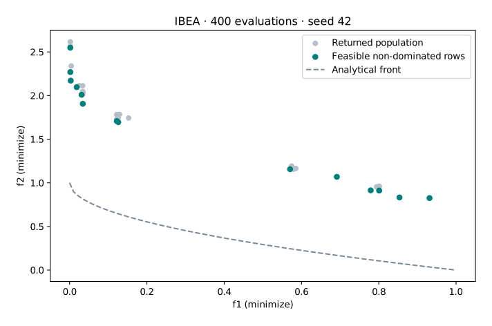
Measured with VAMOS 1.4.0; the observations and provenance retain the inputs and results.
Understand the configuration
| Setting | Meaning in this example |
|---|---|
indicator("eps") |
Uses VAMOS’s epsilon-based fitness path. |
kappa(1.0) |
Controls scaling in the indicator-to-fitness transformation; it is not an evaluation budget or tolerance. This lesson sets 1.0; the default is 0.05, the value of Zitzler and Künzli [1]. |
| SBX + polynomial mutation | Real-coded variation with mutation probability 1/10. |
| Tournament selection | Selects parents using the computed fitness. |
Interpret the result and its limits
Each X row aligns with the same F row. This lesson explicitly requests population mode, then computes the feasible non-dominated subset separately. All objectives are minimized. A non-dominated row is only non-dominated among the available rows; it need not be Pareto optimal. The retained observations contain the actual arrays and configuration.
IBEA normalizes each objective over the population before computing either indicator, as adaptive IBEA does [1]. - Units: a positive affine change of the units of any objective leaves its selection unchanged. - Limitation: solutions far behind the others widen the normalization range and slow convergence on multimodal problems. - Quality: do not infer superior quality from the indicator name. - The figure: it reports objectives in their original units. It does not show a hypervolume-optimized run.
This run has no constraints. Before using a constrained or discrete problem, check the capability matrix and constraint convention. Preserve complete runs through the canonical lifecycle; the teaching JSON is not a replay bundle.
Try one controlled change
Change only kappa to 0.5, preserve the seed and budget, and inspect the result. For a conclusion, repeat the experiment and use a common externally defined measurement protocol.
Next: use T06 to turn this example into a reproducible comparison.
References
[1] Zitzler, E., and Künzli, S. (2004). Indicator-Based Selection in Multiobjective Search. Parallel Problem Solving from Nature — PPSN VIII.