SMS-EMOA
Hypervolume contribution provides the environmental selection criterion: candidates compete through the objective-space volume they add relative to a reference point [1]. This steady-state example makes that point explicit.
Goal: run the stable public API in VAMOS 1.4.0, interpret its returned population, and identify which settings control this mechanism.
Capability matrix · Exact configuration reference · Setup and recorded evidence
Run the example
Prerequisite: complete T01 and the coverage setup. The protocol uses ZDT1, 10 real variables, 2 objectives, population 40; 400 evaluations; NumPy; seed 42. Initial evaluations count towards the budget. Settings are illustrative, not tuned.
python smsemoa.py
python smsemoa.py --output smsemoa-local.svg
The second command reruns the same protocol and requires Matplotlib. Use a new filename.
Complete runnable script
"""Verified VAMOS 1.4.0 lesson: smsemoa. See coverage-setup for dependencies."""


def execute_example(problem, algorithm, config, budget, seed=42, engine="numpy"):
    import numpy as np

    from vamos import OptimizationResult, optimize

    result = optimize(problem, algorithm=algorithm, algorithm_config=config, max_evaluations=budget, seed=seed, engine=engine)
    G = result.data.get("G")
    if getattr(problem, "n_constraints", 0) and G is None:
        raise ValueError("Declared constraints are missing from the returned result.")
    feasible_rows = np.arange(len(result.F)) if G is None else np.flatnonzero(np.all(G <= 0, axis=1))
    if len(feasible_rows):
        feasible = OptimizationResult({"X": result.X[feasible_rows], "F": result.F[feasible_rows]})
        front, local = feasible.front(return_indices=True)
        front_rows = feasible_rows[local]
    else:
        front, front_rows = np.empty((0, problem.n_obj)), np.empty(0, dtype=int)
    print(f"Algorithm: {algorithm}; encoding: {problem.encoding}; backend: {engine}; seed: {seed}")
    print(f"Returned X: {result.X.shape}; F: {result.F.shape}; result mode: population")
    print(f"Feasible rows: {len(feasible_rows)}/{len(result.F)}; feasible non-dominated rows: {len(front)}")
    print(f"Evaluations: {result.data['evaluations']}")
    return {
        "problem": problem,
        "algorithm": algorithm,
        "config": config,
        "result": result,
        "feasible_rows": feasible_rows,
        "front": front,
        "front_rows": front_rows,
    }


def run_smsemoa(budget=400):
    from vamos.algorithms import SMSEMOAConfig
    from vamos.problems import ZDT1

    problem = ZDT1(n_var=10)
    config = (
        SMSEMOAConfig.builder()
        .pop_size(40)
        .crossover("sbx", prob=1.0, eta=20.0)
        .mutation("pm", prob=1.0 / problem.n_var, eta=20.0)
        .selection("random")
        .reference_point(vector=[1.1, 11.0], adaptive=False)
        .result_mode("population")
        .build()
    )
    return execute_example(problem, "smsemoa", config, budget)


def plot_example(data, output):
    from pathlib import Path

    import matplotlib

    matplotlib.use("Agg")
    import matplotlib.pyplot as plt
    import numpy as np

    output = Path(output)
    if output.exists():
        raise FileExistsError(f"Choose a new figure filename: {output}")
    if output.suffix.lower() != ".svg":
        raise ValueError("Use an .svg output filename.")
    f = data["result"].F
    with plt.rc_context({"svg.hashsalt": "vamos-coverage", "svg.fonttype": "none"}):
        fig = plt.figure(figsize=(7, 4.5), layout="constrained")
        if f.shape[1] == 3:
            ax = fig.add_subplot(projection="3d")
            ax.scatter(*f.T, c="#007f7a", s=22)
            ax.set(xlabel="f1", ylabel="f2", zlabel="f3")
            ax.set_box_aspect((1, 1, 0.85), zoom=0.85)
        else:
            ax = fig.add_subplot()
            ax.scatter(*f.T, c="#b6bec8", s=25, label="Returned population")
            if len(data["front"]):
                ax.scatter(*data["front"].T, c="#007f7a", s=30, label="Feasible non-dominated rows")
            labels = {
                "WeldedBeamDesignProblem": ("Cost (minimize)", "Deflection proxy (minimize)"),
                "FeatureSelectionProblem": ("Validation error (minimize)", "Feature count (minimize)"),
                "HyperparameterTuningProblem": ("Validation error (minimize)", "Complexity proxy (minimize)"),
            }
            xlabel, ylabel = labels.get(type(data["problem"]).__name__, ("f1 (minimize)", "f2 (minimize)"))
            ax.set(xlabel=xlabel, ylabel=ylabel)
            ax.legend()
        if data["problem"].__class__.__name__ in {"ZDT1", "ZDT1Problem"}:
            x = np.linspace(0, 1, 101)
            ax.plot(x, 1 - np.sqrt(x), "--", c="#7c8795", label="Analytical front")
            ax.legend()
        ax.set_title(f"{data['algorithm'].upper()} · {data['result'].data['evaluations']} evaluations · seed 42")
        fig.savefig(output, metadata={"Date": None}, bbox_inches="tight", pad_inches=0.25)
        plt.close(fig)
    output.write_text("\n".join(line.rstrip() for line in output.read_text(encoding="utf-8").splitlines()) + "\n", encoding="utf-8")


def lesson_cli(function, default_budget=400):
    import argparse

    parser = argparse.ArgumentParser(description="Run a bounded VAMOS example and optionally plot its actual result.")
    parser.add_argument("--budget", type=int, default=default_budget)
    parser.add_argument("--output", help="New SVG filename; requires Matplotlib")
    args = parser.parse_args()
    data = function(budget=args.budget)
    if args.output:
        plot_example(data, args.output)


if __name__ == "__main__":
    lesson_cli(run_smsemoa, default_budget=400)
Recorded output
Algorithm: smsemoa; encoding: real; backend: numpy; seed: 42
Returned X: (40, 10); F: (40, 2); result mode: population
Feasible rows: 40/40; feasible non-dominated rows: 8
Evaluations: 400
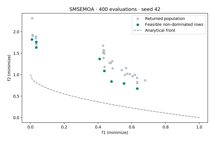
Measured with VAMOS 1.4.0; the observations and provenance retain the inputs and results.
Understand the configuration
| Setting | Meaning in this example |
|---|---|
Fixed reference [1.1, 11] |
Both objectives are minimized; this box covers the chosen ZDT1 domain. It is supplied to selection, not inferred from each result. |
adaptive=False |
Keeps the selection reference fixed throughout this lesson. Adaptive reference behavior is a different experiment. |
| SBX + polynomial mutation | Real-coded variation; mutation probability is explicitly 1/10. |
selection("random") |
Parent selection is separate from hypervolume-based environmental selection. |
VAMOS 1.2.0: a vector is used as given and stays fixed, so it cannot be combined with adaptive=True; points outside its box contribute nothing to the hypervolume and are removed first. Without vector, the reference is nadir + offset * (nadir - ideal) of the population and the new child, recomputed at every step unless adaptive=False. offset (default 1.0) is therefore a fraction of each objective's range, the reference 1 + offset of the normalized objectives, and the selection does not depend on the objective units. In VAMOS 1.1.0 and earlier, offset was added to the maximum in objective units, so rescaling one objective changed which solutions survived. A vector was raised to that maximum plus offset and, with the default adaptive=True, replaced after the first step. The recorded output above uses this lesson's [1.1, 11.0] as given.
VAMOS 1.3.0: reference_point(rule="jmetal") uses the reference point of jMetal's and Evolver's SMS-EMOA (SMSEMOAReplacement in jMetal 7.11), so that results can be compared with theirs: each coordinate is the worst value of the population and the new child times 1.1, or divided by 1.1 when that value is negative, recomputed at every step. The default rule, "relative", is unchanged. The two differ in three ways:
"relative" (default) |
"jmetal" |
|
|---|---|---|
| Coordinate | worst value + offset × (worst − best) |
worst value × 1.1, or ÷ 1.1 when negative |
| Margin above the worst value | offset (default 1.0) times the objective's range |
10% of the worst value when it is positive, about 9% of its magnitude when negative, none when it is 0 |
| Rescaling or shifting an objective | rescales or shifts the reference with it: the same solutions survive | rescaling keeps the survivors; shifting the objective changes the margin and can change them |
With jMetal's rule the reference lies close to the worst values, so the extreme solutions of the last front contribute less than with the default offset=1.0, and with a worst value of 0 they contribute nothing along that objective. The rule takes no vector or offset, and is always adaptive.
VAMOS 1.2.0: with constraints, SMS-EMOA removes the most violated solution while any is infeasible. constraint_handling replaces that rule by another of jMetal's constraint-handling techniques, such as epsilon-constrained or stochastic ranking: the technique ranks the population and the new child, and the least hypervolume contributor of its last front leaves. See choose a constraint-handling technique.
VAMOS 1.2.0: SMS-EMOA creates one child per evaluation, and a generation is pop_size children, as in steady-state NSGA-II. Live callbacks are notified, and an ("hv", ...) target is checked, once per generation rather than after every child; result["generation"] counts these generations. Every child is offered to the external archive as soon as it is evaluated, so a non-dominated child that survival removes as the least contributor is still archived. In VAMOS 1.1.0, every child counted as a generation and the archive received only the survivors.
Interpret the result and its limits
Each X row aligns with the same F row. This lesson explicitly requests population mode, then computes the feasible non-dominated subset separately. All objectives are minimized. A non-dominated row is only non-dominated among the available rows; it need not be Pareto optimal. The retained observations contain the actual arrays and configuration.
Hypervolume depends on the reference point and objective scales. The low budget leaves visible distance from the analytical front. Indicator computation also has a cost; this example does not establish suitability for arbitrarily many objectives.
Every step computes the exact hypervolume contribution of each point in the worst front: with MooCore's hv_contributions when MooCore is installed, otherwise with an exact sweep for two objectives and, for three or more, with one exact hypervolume of the front per point left out. There is no approximation such as Monte Carlo sampling or HypE, so the cost of a step grows exponentially with the number of objectives. Time a short run before planning many-objective experiments, or choose a reference-direction algorithm such as NSGA-III.
This run has no constraints. Before using a constrained or discrete problem, check the capability matrix and constraint convention. Preserve complete runs through the canonical lifecycle; the teaching JSON is not a replay bundle.
Try one controlled change
Increase the budget to 800 with the same seed and reference point. Compare fronts with that fixed box; then repeat several seeds before drawing a quality conclusion.
Next: use T06 to turn this example into a reproducible comparison.
References
[1] Beume, N., Naujoks, B., and Emmerich, M. (2007). SMS-EMOA: Multiobjective selection based on dominated hypervolume. European Journal of Operational Research, 181(3), 1653–1669.